
< Previous | Contents | Next >
4.3.2. Performing Basic Spreadsheet Tasks
Similar to any other spreadsheet application, Calc is used to process numerical information or text in tabular form. It is primarily used for tabulating numerical figures. It also allows you to sort and manipulate data, apply arithmetic, mathematic and statistical functions to data sets and represent the datasets in charts or graphical forms. The following sections describe the instructions to perform some basic spreadsheet tasks in Calc.
Procedure 4.6. Formatting Tables and Cells
To format tables and cells in a Calc spreadsheet:
1. On the Applications menu, point to Office and then click OpenOffice.org Spreadsheet to open a Calc spreadsheet. A new Calc window opens.
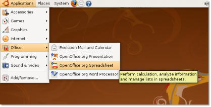
Figure 4.24. Launching Calc
2. Some of the key components of the main Calc window are described below:
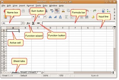
Figure 4.25. The Calc Window
• The Name box contains the cell and the row number, called the cell reference, of the current or active cell.
• The active cell indicates the selected cell currently in use.
• The Function wizard opens the Function Wizard dialogue box.
• The Sum button allows you to calculate the sum of the numbers in the cells that are above the current cell.
• Clicking the Function button inserts an equals sign into the current cell as well as in the input line, making
![]()
it ready to accept a formula.
• The sheet tabs at the bottom of the sheet indicate the number of worksheets present in the current spread- sheet. By default, a new spreadsheet includes three worksheets.
3. After you have entered the required data in the spreadsheet, you can apply different formatting styles to it by selecting from the wide range of options available in Calc. To apply desired formatting to a selected range of cells, on the Format menu, click Cells. The Format Cells dialogue box opens.
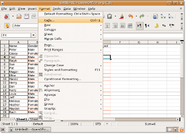
Figure 4.26. Formatting Cells
4. You can use the various options available under the Font, Font Effects and Alignment tabs to specify various formatting attributes for the selected text. Similarly, for assigning formatting attributes to numbers, you can select from a number of pre-defined formats available on the Numbers tab page or define a new one based on your preferences.
The Format Cells dialogue box also provides you with options to add smart borders and vibrant back- grounds to your spreadsheet. It also allows you to select a background colour, from a spectrum of colours, for your otherwise bland and dull spreadsheet.
Define the specifications and click OK to apply the formatting effects.
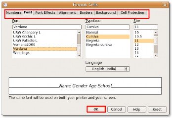
Figure 4.27. Defining Formatting Attributes
5. After you have selected formatting attributes for the selected cell range, you may get a result similar to this one.
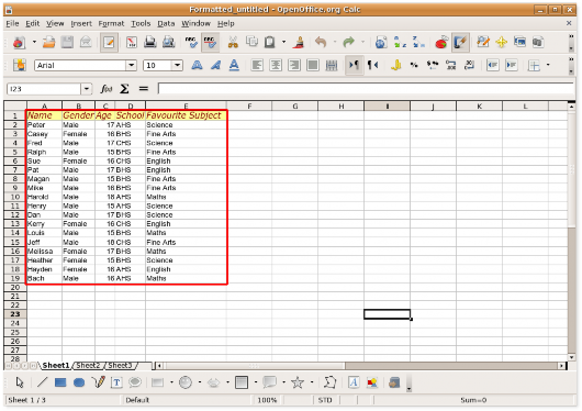
Figure 4.28. The Formatted Spreadsheet
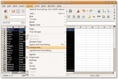
6. Calc provides you with another useful feature, called Autoformat, which enables you to create attractive and professional table designs without undergoing the time-consuming process of selecting cell groups and assigning different formats to them. The Autoformat feature allows you to quickly apply preset formats to an entire sheet or a selected cell range. To apply Autoformat to a sheet or selected cell range, on the Format menu, click Autoformat.
![]()
Figure 4.29. Using Autoformat
7. This displays the AutoFormat dialogue box. To assign a pre-set format to the selected cells, select one from the Format list and then click OK to apply the selected format to the selection.
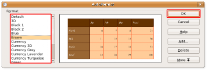
Figure 4.30. Selecting a Format
8. The format of your choice is immediately applied to the selection, and you get an attractive and fully formatted table with very little effort.
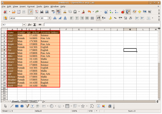
Figure 4.31. The Formatted Table
Entering Values and Formulas. A formula is a spreadsheet function, complete with arguments, entered in a cell. All formulae begin with an equal sign and may contain number, text and, in some cases, other data such as format details. The formulae may also contain arithmetic operators, logic operators or function starts.
Table 4.1. Calc Formulae
Formulae =SUM(A1:A11) | Description Calculates the sum of the cells A1:A11 |
=EFFECTIVE(5%;12) | Calculates the effective interest for 5% annual nominal interest with 12 payments a year |
=B1*B2 | Displays the result of the multiplication of B1 and B2 |
=C4-SUM(C10:C14) | Calculates C4 minus the sum of cells C10 to C14 |
The quickest way to enter a formula is to type the formula either in the cell where you want the result to display or in the Input Line on the Formula bar. You can also use the Function wizard, which helps you interactively create formulae.
Procedure 4.7. To enter a formula using the Function wizard:
1. In your spreadsheet, select the cell where you want the formula to be inserted. To allow the Function wizard to guide you through the creation and application of a formula, on the Formula bar, click Function Wizard. This opens the Function Wizard dialogue box.
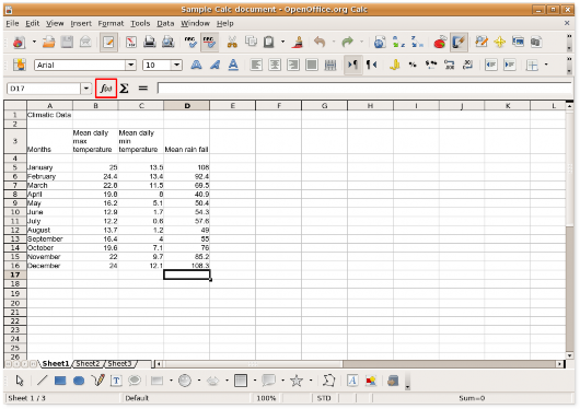
Figure 4.32. Launching Function Wizard
2. You can see the entire range of functions listed in the Functions list box. You can also select one catego- ry from the Category drop-down list to display the functions listed under that category. Find the desired function from the Functions list, and click to select it. You notice that the Function Wizard dialogue box provides you some information about the selected function to guide you through your selection. After selecting the function, click Next to proceed with the task of entering a formula.
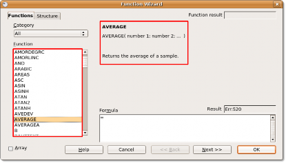
Figure 4.33. Selecting a Function
3. Now, you need to specify the numbers to which you want to apply the formula. To select the numbers, you need to go back to the worksheet.
Click the Shrink button to shrink this dialogue box and return to the worksheet.
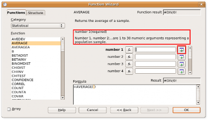
Figure 4.34. Shrinking the Function Wizard Dialogue Box
4. The Function Wizard dialogue box shrinks to allow you to view the worksheet. To select the cell range, hold down the SHIFT key and use the mouse to select the cell range containing the desired numbers.
After selecting the cells, you can go back to the Function wizard by clicking the Maximize button.
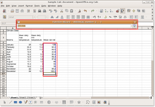
Figure 4.35. Selecting the Cell Range
5. The cell reference for the selected cell range automatically appears in the number 1 box and the applied formula, complete with arguments, appears in the Formula box at the bottom of the dialogue box. To complete the task of entering a formula, click OK.
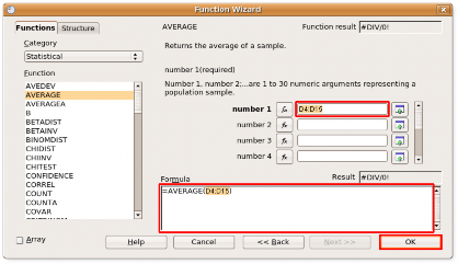
Figure 4.36. Applying the Formula
6. The solution appears in the cell where you had applied the formula.
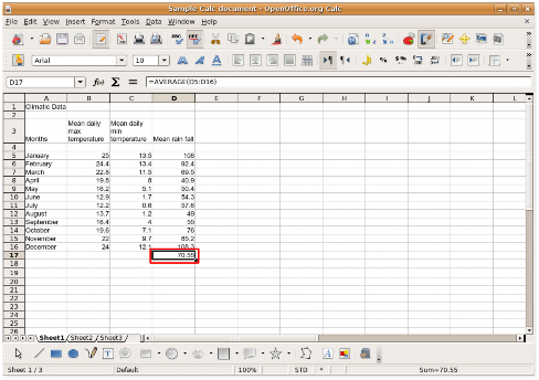
Figure 4.37. Final Output
Inserting Charts. You can present your data in the form of charts or graphs to compare your data series visually and view trends in the data. Calc offers you a number of ways to represent spreadsheet data graphically.
Procedure 4.8. To insert a chart in your spreadsheet:
1. Open a spreadsheet containing data and row and column headings, and select the data to be included in the chart. Then, on the Insert menu, select Chart. The Chart Wizard dialogue box appears.
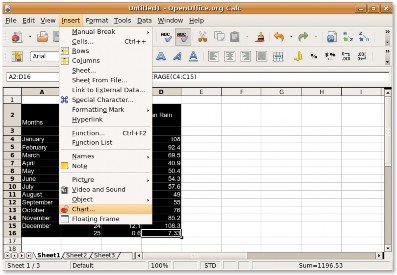
Figure 4.38. Launching the Chart Wizard
2. On the first page of the Chart wizard, you can select the chart type and preview the chart output. Calc allows you to select from a wide range of 2D and 3D charts. You may decide to follow the rest of the instructions of the Chart Wizard by clicking Next or you can click Finish to insert a chart in your document.
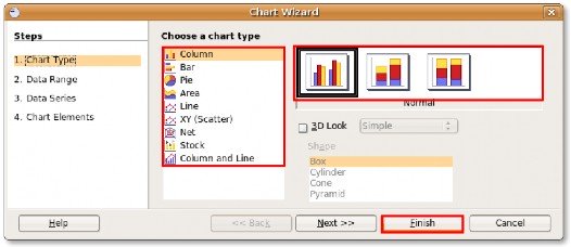
Figure 4.39. Selecting the Chart Type
3. The chart is inserted at the specified location in your spreadsheet. You can now move and resize the chart and edit it further to suit your requirements.
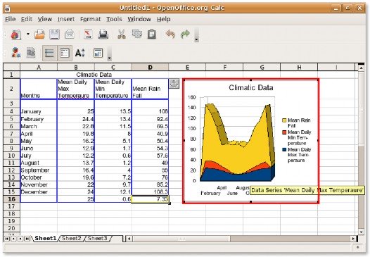
Figure 4.40. The Inserted Chart
Exporting Spreadsheets to PDF. Like the other OpenOffice.org applications, you can export your spread- sheets from Calc as PDF files. With OpenOffice.org you do not need any additional third party software to convert your documents into PDF format.
Procedure 4.9. To export your spreadsheet as a PDF:
1. On the File menu, click Export as PDF. The Export dialogue box appears.
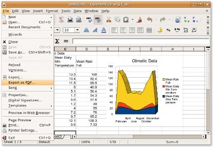
Figure 4.41. Exporting Spreadsheet as PDF
2. The four tabbed pages in this dialogue box allow you to define options, such as the pages to be included in the PDF, the type of compression to be used and the level of security to be assigned to the file. After defining these specifications, click Export to continue.
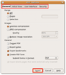
Figure 4.42. Defining PDF Options
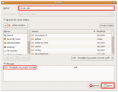
3. Provide a file name for your spreadsheet and navigate to the directory where you want to save it. Click
Save to export the spreadsheet as a PDF file.
![]()
Nice to Know:
Figure 4.43. Saving as PDF
To discover an Easter Egg tucked away in Calc, click within any of the cells of your spread- sheet, type = GAME("StarWars") and start playing right away.
4. Your spreadsheet is now displayed as a PDF file.
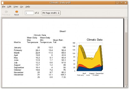
Figure 4.44. The PDF file